
| 일 | 월 | 화 | 수 | 목 | 금 | 토 |
|---|---|---|---|---|---|---|
| 1 | 2 | 3 | 4 | 5 | ||
| 6 | 7 | 8 | 9 | 10 | 11 | 12 |
| 13 | 14 | 15 | 16 | 17 | 18 | 19 |
| 20 | 21 | 22 | 23 | 24 | 25 | 26 |
| 27 | 28 | 29 | 30 |
- 1st Law of politics
- mechanism of politics
- Regime Change
- Political Change
- the 3rd Law of politics
- Mathematical Model of political science
- Mathematical Model of politics
- Differences in Individual Abilities and Tendencies
- power and organization
- Cohesion Force
- political organization
- Task Delegates of the Ruler: Inner Circle
- the 2nd law
- Samjae Capacities
- Political Regimes
- Political Regime
- Political power
- survival process theory
- Canonical Politics
- Orderliness of Choice
- new political science
- Value Systems
- politics and war
- political phenomena
- Order of Choice
- Operation of the 2nd Law
- politics of Inner Circle
- politics
- Power
- Samjae Capacity
- Today
- Total
New Political Science
a. ㉡ Schematic Understanding of the 3rd Law 본문
a. ㉡ Schematic Understanding of the 3rd Law
Political Science 2023. 12. 14. 02:31㉡ Schematic Understanding of the 3rd Law
In [Diag.3.C.1] above, the economic regime(political regime in the economic sector) moved from a low level to a high level, which can be understood as an increase in tenant farming fees. However, this diagram does not show the interaction of many factors that affect political changes. Therefore, to diagram all factors interacting with political changes, each of these factors must be abstracted into simple points or rectangles on a coordinate plane and combined.
Let me look back at [Diag.2.A.6]. In this diagram, if the size of the political capacity of political actors a and b changes, the size of their power also changes. Moreover, if the political capacity of many political actors changes, the rule system (political regime) determined by their power relations also changes. The following diagram represents the relationships of factors that affect such changes.
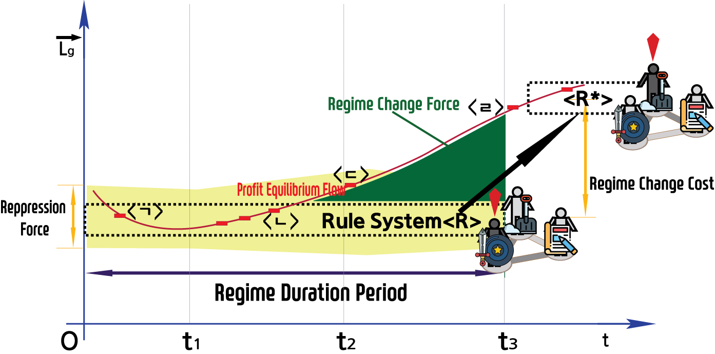
The basic framework for the idea being presented, which concerns the temporal changes in political regimes and power, is the - coordinate space that shows the changes in political regimes (rule systems) over time - which will be referred to as the "tL-space." The horizontal axis represents time(t), which flows from the past to the future, while the vertical axis represents the interests or survival capacity( \( \vec{L} \) ) of various factions within a political organization(g). In this diagram, we assume that the degree of advantage to two types of political actors (such as "haves" and "have-nots") distinguished by a one-dimensional quantity is indicated.
In interpreting the vertical axis, it can be set that a larger value indicates a greater advantage for the haves, while a smaller value indicates a greater advantage for the have-nots. Alternatively, a larger value can be set to be more advantageous for conservative forces, while a smaller value is more advantageous for progressive forces. Of course, it is also possible to set it in the opposite direction. (In this Diagram, it was assumed that there is only one point of contention for changes in the political regime, but there may be more. When there are points of contention, the tL-space will become an dimensional space.)
The focus here is on the political regime, represented by a dotted black square in the diagram(rule system R). At a specific point in time(t), the rule system is a segment of a vertical line at t, and as it continues over time, it becomes a square. The vertical length of the rule system represents the set of rules that political actors with the capacity( \( \vec{L} \) ) covered by that segment of the vertical line desire (which is of the highest profit to them). For example, if the L-axis represents tenant farming fees, and the rule system extends from 100 to 200 won, the regime is one that allows all values between 100 and 200 won for tenant farming fees. All rule systems have some level of vertical length, which can be long or short, representing the "system flexibility"(Flx). Additionally, rule systems persist over time, which is represented by the horizontal length of the rule system(R). This represents the "regime duration period(T)."
In addition, all rule systems have a constraint force[Ch.2.6b]. It is the force that compels actions outside of the rules, namely, actions (or capacities) that do not benefit those who possess specific capacities to enter into the rule system. This force is called "repression force( \( \vec{S_{TB}} \) )" and is marked by the yellow area spreading up and down in the rule system shown in [Diag.3.C.2]. The state power imposes penalties on actions outside of the regime.
On the other hand, we can assume a virtual rule system in which the understanding of political actors is actually adjusted to the best state. Let me call the point representing this rule system the "profit equilibrium condition" and the temporal change of these points the "profit equilibrium flow(At)". In the diagram, the profit equilibrium flow is represented by the red curve in the above diagram, and the profit equilibrium conditions are indicated by <ㄱ>, <ㄴ>, <ㄷ>, and so on, on the curve. In addition, let me call the slope of the profit equilibrium flow the "social change rate". The profit equilibrium conditions change rapidly as the social change rate increases, and consequently the slope of the profit equilibrium flow also increases.
In the above diagram, political regime change refers to the movement from one rule system(R) to another rule system(R*). This phenomenon arises from the force that seeks to change the regime, which we call 'regime change force( \( \vec{H} \) )'. The regime change force( \( \vec{H} \) ) is the profit obtained when disposing of the existing rule system(R) and creating a new rule system(R*), and the amount of this profit is the area created by the height difference of the space between the profit equilibrium condition at a given point and the rule system(R) in the diagram [Diag.3.C.2]. This is also the sum (or integral) of accumulated losses over time.
On the other hand, the cost of changing the rule system is referred to as the "regime change cost( \( \vec{C} \) )." Generally, regime change cost is the most important reason why people do not change the rule system. In [Diag.3.C.2], the regime change cost is indicated by an arrow that shows the movement from the current rule system(R) to the new rule system(R*). The magnitude of this value is intuitively proportional to the difference in value between the two rule systems in the tL-coordinate space, but it is actually influenced by many other factors. Meanwhile, the regime change cost and the repression force( \( \vec{S_{TB}} \) ) combine to form resistance force( \( \vec{R_{ST}} \) ), which resists regime change.
When the profit resulting from regime change increases, demand also increases, eventually leading to the emergence of political force. At that point, the existing rule system(R) disappears and a new rule system(R*) becomes a reality. This is regime change, which is also political change. Naturally, regime change occurs when regime change force surpasses resistance force.
In order to visually represent and understand political phenomena using this diagram, the following expression method can be chosen, which will be helpful in applying this schematic to various aspects.
[Def. 3.1] The transformation from the existing rule system(R) to a new rule system(R*) is called regime change (R→R*). The larger the difference in the L (vertical) value between R and R*, the greater the "regime change".
[Def. 3.2] The difference in L (vertical) value between the profit equilibrium condition, which is a point of the profit equilibrium flow(At), and the rule system(R) indicates the discrepancy between the rule system and reality. The greater this discrepancy, the greater the loss for the entire political organization(g).
[Def. 3.3] The regime change force( \( \vec{H} \) ) is the sum (i.e. area) of the distances between the profit equilibrium condition and the rule system.
[Def. 3.4] The regime change cost( \( \vec{C} \) ) is the cost of moving from the previous rule system to the new rule system.
[Def. 3.5] The slope of the profit equilibrium flow(At) indicates how quickly people's practical interest relation structure changes (social change rate).
[Def. 3.6] The vertical width of the rule system(R) space itself represents regime flexibility(Flx). Regime flexibility is also the complexity of the rule system.
[Def. 3.7] The longer the vertical length( \( \vec{S_{TB}} \) ) of the yellow area surrounding the rule system(R) space, the stronger the repression force.
'Mechanism of Politics' 카테고리의 다른 글
| (2) Interpretation and Examples of the 3rd Law (0) | 2023.12.14 |
|---|---|
| b. Formulation of the 3rd Law (0) | 2023.12.14 |
| a. ㉠ Detailed Content of the 3rd Law (0) | 2023.12.14 |
| C. (1) Intuitive Explanation Through Diagrams (0) | 2023.12.14 |
| c. Mathematical Model and Implications of the 2nd Law (0) | 2023.12.14 |
